Importing from Google Sheets with Quickstarts
You can use Quickstarts to automatically import structured data from Google Sheets up to 10,000 rows.
Steps to import from Google Sheets with Quickstarts
The steps to import from Google Sheets are:
Find the URL of your Google Sheet.
See Finding the URL of a Google Sheet for details.
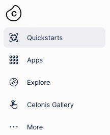
Run Quickstarts.
Depending on your configuration, you might see it in the left navbar. Otherwise, you can access Quickstarts through Studio.
Click the Google Sheets tile.
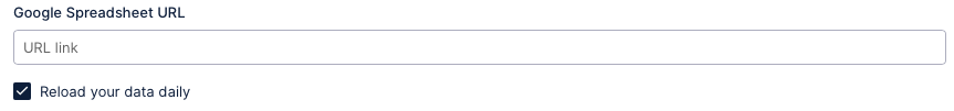
Enter the URL of your sheet.
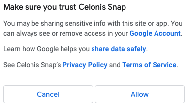
Give Celonis permission to access your sheet.
At this point, Celonis will automatically extract the data from your spreadsheets.
Note
When you allow access, Celonis Platform can read the data but the data is still entirely secure and private. No one outside your organization can access the data.
If the Google sheet has more than one worksheet (that is, more than one tab), you need to select which one you want to import.
You can search for a tab by name, or select the one you want from a list.
Sign in and click Allow to give Quickstarts access to the sheet.
Select the sheet you want to work with. and click Next.
Google Sheets can have multiple spreadsheets. You can upload one at a time.
Check that the data types are correct.
When Quickstarts looks at a file, it attempts to understand the data types. Usually it's successful but it's impossible to get it right every time. For example, the date and time stamp looks like a string data type but, really, it's a datetime data type. So it's a good idea to check manually.
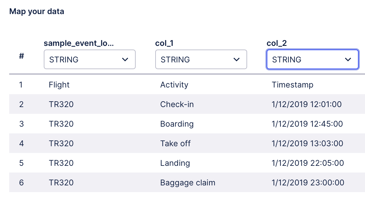
Click on the column that contains the Case ID.
This is simply to show Quickstarts where it can find the Case ID.
Click on the column that contains the Activity name.
Click on the column that contains the Timestamp.
In this example, it would be: dd/MM/yyyy HH:mm:ss.
Read more about date formatting.
Choose a Sorting column and click Next.
We'll use the to organize your data. You can ignore this step if you want to.
Quickstarts can now process your data. You're all set. It does all the heavy lifting for you. When it has finished, you can move on to examine your data in an easy-to-use component of Celonis Platform called Business Miner, to start gaining actionable insights.
What happens now?
When Quickstarts completes the import of your data, you're all set to go!
You'll land in a ready-to-use Business Miner exploration. Select the question that you want to answer and start mining! Take a look at the Business Miner documentation to discover all the things you can do next.
Business Miner uses a Process Workspace. A Process Workspace is where all Business Miner content is stored. It’s also where you collaborate with colleagues. To make life easy, Quickstarts automatically creates a Process Workspace for you.
Finding the URL of a Google Sheet
It's easy to find the URL of a Google Sheet:
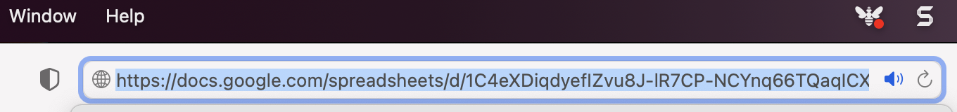
Open the Google Sheet.
Copy the entire URL from the address bar to the clipboard.
You can now paste the URL anywhere you need to.
Important
Any references to third-party products or services do not constitute Celonis Product Documentation nor do they create any contractual obligations. This material is for informational purposes only and is subject to change without notice.
Celonis does not warrant the availability, accuracy, reliability, completeness, or usefulness of any information regarding the subject of third-party services or systems.