PQL performance optimization guide
Description
As the complexity of the PQL queries grows, you might experience a decline in query performance. A noticeably prolonged query runtime is the main sign of bad performance. On the front-end side, when looking at a dashboard, it might happen that some of the components take longer to load or, in the worst case scenario, if the query gets rejected/fails - the view does not load at all.
For this reason, it might be helpful for you to learn some basics about what happens in the background when a PQL query is executed. We will also cover some good practices which you should use when writing queries or creating dashboards.
Understanding the connection between front-end and PQL queries
From front-end components to queries
What do our users' dashboards look like? They can be very diverse. In Celonis we have created plenty of components which you can add to your dashboard to describe your process in a way that best fits your needs. This means you can choose between many charts and tables, process or KPI components. In addition, you could decide to define a specific component filter or sheet filter.
What is important to understand is that whatever components you use to design a dashboard - all of them will translate into one or multiple PQL queries. Depending on the complexity, they can take more or less time to execute. Simple front-end components and the corresponding query:
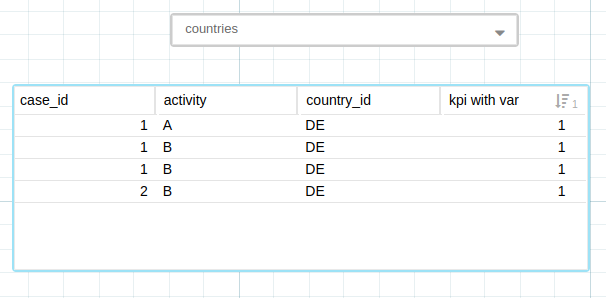
FILTER KPI ("kpi_formula", VARIABLE('DE')) = 1TABLE( "activities"."case_id" AS "case_id", "activities"."activity" AS "activity", "activities"."country_id" AS "country_id", KPI("kpi_formula", VARIABLE ('DE')) AS "kpi with var" ) ORDER BY KPI("kpi_formula", VARIABLE ('DE')) DESC LIMIT 400;Designing performant Views and Boards
What choices could you make in your dashboard design to improve the performance? More complex dashboards mean more queries that need to be executed which in turn often leads to longer runtimes. The solution is - try to keep your boards as clean and simple as possible.
Note: If there is more data that you want to explore, but your dashboard is already over-crowded or loading too slowly - try to spend some time thinking about the information you want to see, try to group it into meaningful sections, and create separate dashboards from there.
Additional tips that could help improve your dashboard's performance:
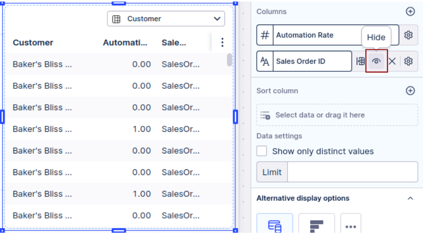
Hide columns by default and only show them when needed. This lets you concentrate on the necessary information and also improves the performance of your dashboards. This is where you can find these options in Analysis and Views:
Analysis (under General Options)
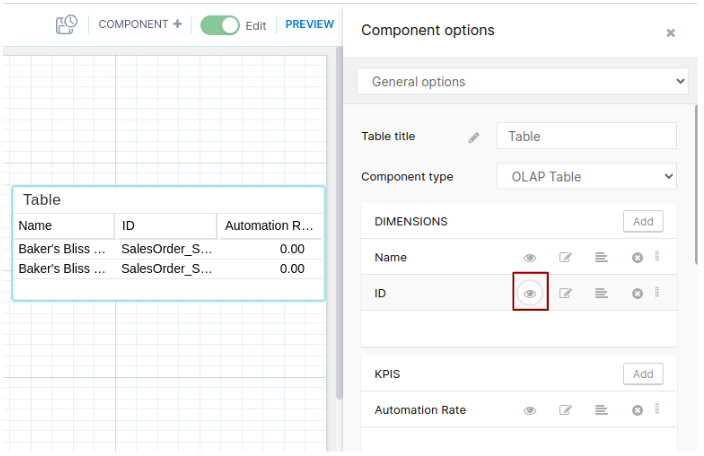
View (under Settings > Columns)
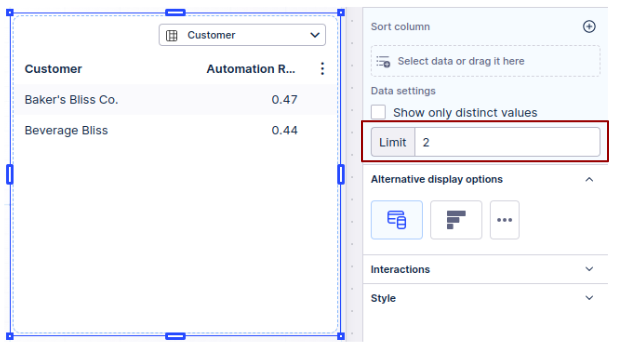
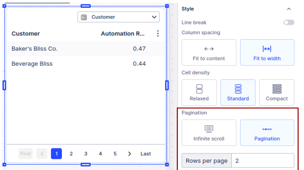
When you have large columns that you want to analyze - try not to visualize columns in their entirety in your dashboard. Instead, try using the "limit" option to show only a specific number of rows. Another option to use is "scrolling" (the alternative option in Analysis after "limit") or "pagination" (in Views) - this way you will be able to view your data by scrolling or clicking through pages. When you enable these options, your data gets loaded in smaller batches making your front-end experience smoother. This is where you can find these options in Analysis and Views:
Analysis (under Advanced Options)
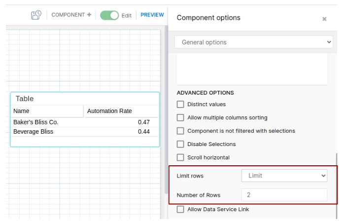
View limit (under Settings > Data settings)
View pagination (under Settings > Style > Pagination)
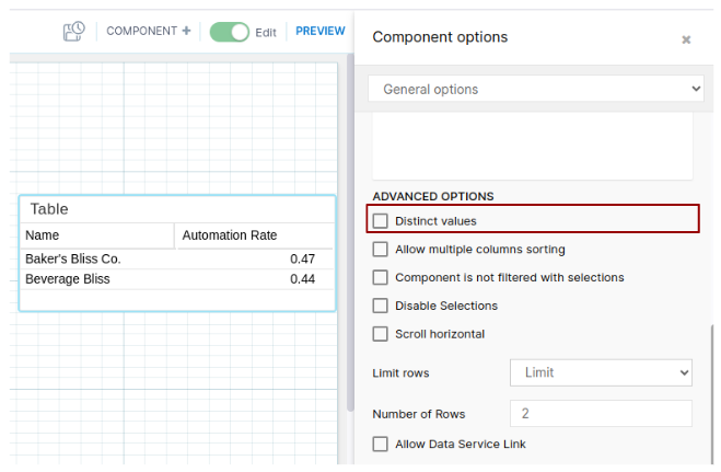
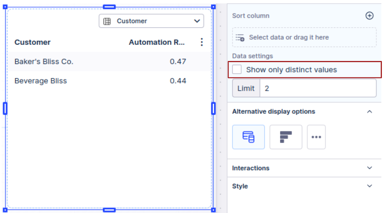
Avoid using the distinct values option when not absolutely necessary. Remember that the rows are often already distinct, especially so when the number of columns is high. This is where you can find the "distinct values" option in Analysis and Views:
Analysis (under Advanced Options)
View (under Settings > Data settings)
Understanding caching
What is caching
To make queries execute faster we use caching. A cache is a temporary storage. Caching is the process of storing the result of a query (or parts of the query) in cache so that the same query can be answered in the future without being executed again. The result is then just recalled from the cache.
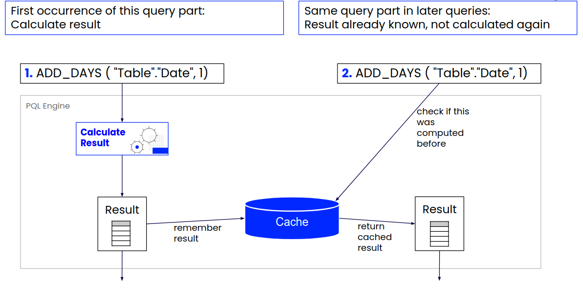
Note: Loading results from cache may not always be instantaneous. In order to make the best usage of the limited cached capacity, cached columns that are not accessed for 5 minutes are compressed to preserve space. In addition, if they are not accessed for 30 minutes they get moved from the in-memory cache to disk. This means that you might experience a delay when accessing cached results that have not been used for a while, because they have to be decompressed or even read from disk before they can be used again.
Cache warmup
Cache warmup happens at the end of the data model load whenever new data is loaded. The aim of cache warmup is to offer the fastest possible query runtime. What this means is that we gather the statistics about the most computationally-intensive queries and we execute those queries right after the data model load. The results are then stored in cache and can be recalled anytime, which offers a smooth front-end experience.
Note: The data model load will not be shown as complete until the cache warmup is finished as well. This can be very important if you have frequent data model loads. In that case it makes sense to think about the tradeoff between the time needed to finish the data model load and to run the queries afterwards. Longer query warmup will in most cases make the query execution more efficient, but it is not a "one-size-fits-all" and it might not make sense for every single data model.
We can enable or disable your query warmup upon request. Also upon request, we can adjust your query warmup duration and make it longer or shorter.
Breakdown of the query runtime
Query runtime is the time between sending the query and receiving the result.
Runtime consists of multiple steps, however the execution of the query usually takes the longest.
The time of execution can increase if the query is very long, if queries are written so that they cannot be cached or if some of the less performant operators are used.
Note that it can happen in extreme cases that other steps take a significant amount of time as well. Parsing and compilation can take more time, for example, when the query is extremely long.
Note: Long queries are often generated when you overuse or excessively nest the KPIs. In PQL we have implemented optimizations to improve the execution of queries with KPIs. However, it is good practice to keep in check what your KPIs are supposed to calculate as deep nesting can often be simplified.
Steps performed during the query runtime and the average percentage each step takes in the overall runtime:
Step | AVG [%] |
|---|---|
Routing | 4.1 |
Parsing | 0.9 |
Compilation | 5 |
Execution | 90 |
Writing cache efficient queries
When exactly do the results of your query get cached? When the computation of the result does not depend on the current filter state.
Some functions take filters into account and others do not.
Standard aggregation (for example, AVG) take filters and selections into account. Values that are filtered out are not a part of the result. That means that the results of standard aggregations are not cached.
On the other hand, PU-functions (for example, PU_AVG) ignore filters. This means that if the filter changes, the result of a PU function will not be affected and also will not be recalculated - the result of a PU-function can be cached. Very important to note here is that caching PU-functions becomes impossible once you decide to use another operator inside the PU function which takes filters into account. This table shows some examples of queries which are cached and some which are not cached. The last example shows the previously mentioned example when the cacheability stops because of FILTER_TO_NULL used inside the function.
Query | Cached? | Reason |
|---|---|---|
"Table"."Price" + "Table"."Tax" | cached | Filter independent operator, so it gets cached. |
CASE WHEN "Table"."Type" = 'T1' THEN 1 ELSE NULL END | cached | If CASE WHEN statements are filter-independent, then the result of CASE WHEN will also be cached. |
AVG("Table"."Price") | not cached | Standard aggregations take filters into account, so the result will not be cached here. |
PU_AVG("TargetTable", "Table"."Value") | cached | PU-functions do not take filters into account, so this will be cached. |
PU_AVG("TargetTable", FILTER_TO_NULL("Table"."Value")) | not cached | FILTER_TO_NULL makes PU functions filter-dependent, so this will not be cached. |
For complex expressions composed of filter-dependent and filter-independent operators, only sub expressions that do not contain a filter-dependent operator will be cached.
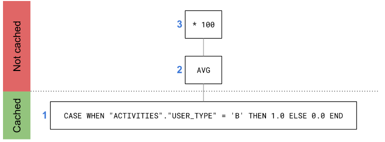
Consider the following expressions:
100 * AVG (CASE WHEN "ACTIVITIES"."USER_TYPE" = 'B' THEN 1.0 ELSE 0.0 END)
CASE WHEN is filter independent and will be cached. However, AVG cannot be cached and therefore the surrounding multiplication cannot be cached:
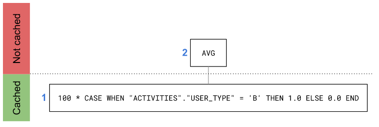
A rule of thumb here is to avoid computations on the result of a non-cached operator whenever possible. In this case, we can get the same result by performing the multiplication before the AVG:
Recalculating operations on filter changes
Some operators require recalculation whenever a filter changes. This can have a negative effect on performance. The following operators fall into this category:
Filter propagation
Filter propagation is necessary if there are one or more tables on which a filter is applied, which are not the same as the result table. In that case we propagate the filters to the result table along the join graph.
Excessive filter propagation can have a negative impact on performance. This is the case for the UNION_ALL operator with an increased number of input arguments. Here filters set on tables joined to any input argument are propagated to the UNION_ALL table.
For this reason, even though the UNION_ALL operator allows up to 16 input arguments, it is recommended to use as few inputs as possible.
Using PU-functions effectively
As mentioned before, PU-functions are mostly cached. Additionally, they can be nested into other aggregations or other PU-functions. This gives better query performance. Take a look at the example below.
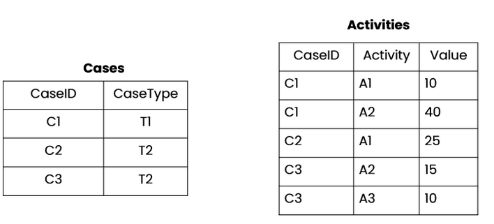
If we want to calculate a maximum of all activities per CaseType, we could choose one of these options:
Option 1 | Option 2 |
|---|---|
"Cases"."CaseType", MAX("Activites"."Value") | "Cases"."CaseType", MAX(PU_MAX("Cases","Activites"."Value")) |
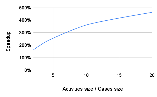
Option 2 allows you to lower the dimension you are calculating on by first pulling up the values to the table representing cases. The non-cached MAX operator is then only calculated on the "Cases" table, instead of on all of the values in the "Activities" table.
Since activity tables are usually much larger than case tables, this can greatly reduce the runtime of the query. The following graph shows the speedup factor depending on how large the "Activities" table is compared to the "Cases" table:
Understanding the effect of FILTER_TO_NULL
FILTER_TO_NULL is used to make operators that otherwise ignore filters, aware of them. FILTER_TO_NULL by itself is not slow, but as a result of using it, all subsequent computations cannot be cached and need to be recomputed every time a filter changes, which causes a drop in performance.
For this reason, you should not use FILTER_TO_NULL unless it is unavoidable. If you cannot avoid using FILTER_TO_NULL, then you should try to use it at the latest possible point in the query, as that might allow the caching of at least some of the operations which happen before FILTER_TO_NULL.
Consider the following two expressions that always have the same result:
PU_FIRST ( "Table1", UPPER ( FILTER_TO_NULL ( "Table2"."Column1" ))) | Whenever you decide to change the filter state, both the UPPER and PU_FIRST operators have to be recomputed because they occur after the FILTER_TO_NULL. |
PU_FIRST ( "Table1", FILTER_TO_NULL ( UPPER ( "Table2"."Column1" ))) | By moving the UPPER operator inside the FILTER_TO_NULL, we can now cache the result of UPPER. If you change the filter, the PU_FIRST operator has to be recomputed. |
When using PU-functions you have the option to add a FILTER parameter as one of the arguments of the operator call. Try to go for this option over using FILTER_TO_NULL directly on the input column. When adding the filter parameter to a PU-function, the result will be cached as long as the filter parameter is not modified.
Bad for performance | A better alternative |
|---|---|
FILTER "caseTable"."caseID" > 2; | PU_MAX ( "companyDetail" , "caseTable"."value" , "caseTable"."caseID" > 2 ) |
PU_MAX ( "companyDetail" , FILTER_TO_NULL("caseTable"."value") ) |
Note: You should always avoid using FILTER_TO_NULL in a FILTER statement. FILTERs might be propagated to multiple queries and if there is a FILTER_TO_NULL in the FILTER statement, all of those queries will have to be recalculated and the information will not be cached efficiently.
Preferring performant operations
Different PQL operators can often be used to compute the same result. However, the runtime of these operators can differ considerably. In the following sections, we use the term "expensive" to express that an operation/function has a longer runtime. Equivalently, we refer to more performant functions as "less expensive". Choosing the less expensive function can help you improve the performance of your queries.
Choosing between standard aggregations
While standard aggregations are sometimes used interchangeably, some are less expensive than others. We can roughly divide aggregations into two categories:
Simple Aggregations | COUNT, MIN, MAX, SUM, AVG, PRODUCT. |
Complex Aggregations | MEDIAN, QUANTILE, MODE, COUNT_DISTINCT, TRIMMED_MEAN. |
Complex aggregations require more steps to be computed and can be quite expensive in comparison. The following graph gives you an idea about how expensive different standard aggregations are:
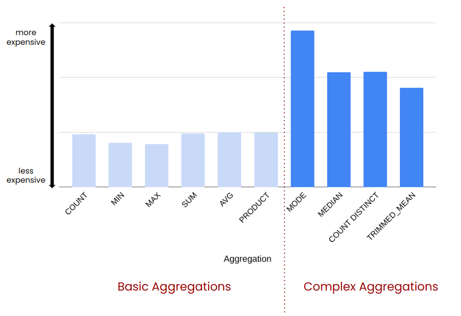
COUNT is significantly less expensive then COUNT ( DISTINCT ). When you have a choice, you should always opt for COUNT.
Example 1:
Table1
Column1: int |
|---|
1 |
2 |
3 |
Column1 is a key column in Table1.
Query1 | COUNT ( DISTINCT "Table1"."Column1" ) |
|---|---|
Query2 | COUNT ( "Table1"."Column1" ) |
COUNT (DISTINCT "Table1"."Column1"): int | COUNT ("Table1"."Column1"): int |
|---|---|
3 | 3 |
When counting a key column, the values are guaranteed to be distinct. In such cases, using DISTINCT is unnecessary.
Example 2:
Table1
Column1: int | Column2: int | Column3: int |
|---|---|---|
1 | 1 | 2 |
1 | 1 | 1 |
1 | 2 | 2 |
2 | 1 | 1 |
Column1, Column2, and Column3 together form a key of Table1.
Query1 | "Table1"."Column1", "Table1"."Column2", COUNT ( DISTINCT "Table1"."Column3" ) |
|---|---|
Query2 | "Table1"."Column1", "Table1"."Column2", COUNT ( "Table1"."Column3" ) |
COUNT (DISTINCT "Table1"."Column3"): int | COUNT ("Table1"."Column3"): int |
|---|---|
2 | 2 |
1 | 1 |
1 | 1 |
If the dimension columns in combination with the argument column form a key of the common table, it is guaranteed that COUNT and COUNT ( DISTINCT ... ) will deliver the same result.
With more dimension columns, this key condition is more likely to be satisfied.
Example 3:
Query1 | "Table1"."Column1", CASE WHEN COUNT ( DISTINCT "Table1"."Column2" ) > 0 THEN 'YES' ELSE 'NO' END |
|---|---|
Query2 | "Table1"."Column1", CASE WHEN COUNT ( "Table1"."Column2" ) > 0 THEN THEN 'YES' ELSE 'NO' END |
COUNT ( DISTINCT "Table1"."Column2" ) > 0 and COUNT ( "Table1"."Column2" ) > 0 are always equivalent. Since Query2 is faster than Query1, using DISTINCT in such cases is unnecessary.
Calculating the MEDIAN needs the data to be sorted. As a result it is significantly more expensive than the AVG operator. When you have a choice, you should always opt for AVG.
Example:
Table1
Column1: int |
|---|
5 |
1 |
5 |
1 |
3 |
MEDIAN ("Table1"."Column1"): int | AVG ("Table1"."Column1"): float |
|---|---|
3 | 3 |
In a uniform or normal distribution, average provides a very good estimation of the median. In such cases you can choose AVG over MEDIAN. However, when data is skewed the result can be way off.
Sometimes the result given by COUNT could be obtained using SUM instead. However, COUNT is less expensive and should be preferred in these situations.
Example:
Query1 | SUM ( CASE WHEN "Table"."Column" = 'A' THEN 1 ELSE 0 END ) |
|---|---|
Query2 | COUNT ( CASE WHEN "Table"."Column" = 'A' THEN 1 ELSE NULL END ) |
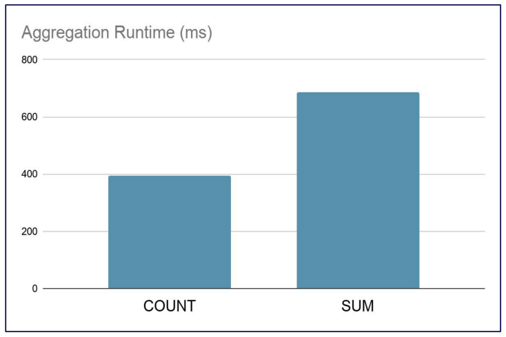
Both Query1 and Query2 give the same result, but Query2 is much faster.
Choosing between PU-functions
Similar to standard aggregations, PU-functions with different cost can be used to compute the same result. Generally the same preferences that apply to standard aggregation, also apply to PU-functions.
Counting only distinct values is significantly more expensive. When possible, you should choose PU_COUNT over PU_COUNT_DISTINCT.
Example 1:
Table1
Column1: int |
|---|
1 |
2 |
Table2
Column1: int | Column2: int |
|---|---|
1 | 1 |
1 | 2 |
1 | 3 |
2 | 4 |
2 | 5 |
Column2 is a key column in Table2.
PU_COUNT ("Table1", "Table2"."Column2"): int | PU_COUNT_DISTINCT ("Table1", "Table2"."Column2"): int |
|---|---|
3 | 3 |
2 | 2 |
When counting a key column, PU_COUNT and PU_COUNT_DISTINCT always have the same result.
Example 2:
Query1 | FILTER PU_COUNT ( "Table1", "Table2"."Column1" ) > 0 |
|---|---|
Query2 | FILTER PU_COUNT_DISTINCT ( "Table1", "Table2"."Column1" ) > 0 |
When the purpose of counting is to check if there is at least one value, using DISTINCT is not needed and just makes the performance worse.
PU_MEDIAN is significantly more expensive than the PU_AVG since it requires sorting. When possible, you should opt for PU_AVG.
Example:
Table1
Column1: int |
|---|
1 |
Table2
Column1: int | Column2: int |
|---|---|
1 | 5 |
1 | 1 |
1 | 5 |
1 | 1 |
1 | 3 |
PU_AVG ("Table1", "Table2"."Column2"): float | PU_MEDIAN ("Table1", "Table2"."Column2"): int |
|---|---|
3 | 3 |
In a perfectly symmetrical distribution like the one in Table2.Column2, the average and the median will be equal.
PU_COUNT is less expensive than PU_SUM. When possible, you should opt for PU_COUNT.
Example:
Query1 | PU_SUM ( "Table1"."Column1", CASE WHEN "Table2"."Column1" = 'A' THEN 1 ELSE 0 END ) |
|---|---|
Query2 | PU_COUNT ( "Table1"."Column1", CASE WHEN "Table2"."Column1" = 'A' THEN 1 ELSE NULL END ) |
Both Query1 and Query2 give the same result, but Query2 is much faster.
Choosing less expensive expressions
In order to compute something, there is often more than one expression that can be used. These expressions could be a single operator or a combination thereof. Following is a list of preferences when there are multiple equivalent options to choose from, based on the performance of each option.
Prefer REMAP_VALUES over CASE WHEN
REMAP_VALUES and CASE WHEN can be used to obtain the same results. However REMAP_VALUES is less expensive than CASE WHEN.
Example:
Query1 | CASE WHEN "Table"."Currency" = 'EUR' THEN 'Euro' WHEN "Table"."Currency" = 'USD' THEN 'US Dollar' ELSE 'Other' END |
|---|---|
Query2 | REMAP_VALUES ( "Table"."Currency", [ 'EUR' , 'Euro' ], [ 'USD', 'US Dollar' ], 'Other' ) |
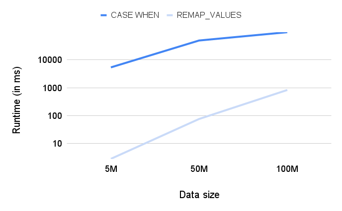
Both Query1 and Query2 give the same result, but Query2 is faster.
Note: you should also prefer REMAP_INTS to CASE WHEN.
The LIKE operator can be used to check for string equality. However, the = operator performs the job in a simpler and less expensive way.
Example:
Query1 | "Activities"."Activity" LIKE 'A' |
|---|---|
Query2 | "Activities"."Activity" = 'A' |
Both Query1 and Query2 give the same result, but Query2 is faster.
Note: you should also prefer != over NOT LIKE when possible.
The IN_LIKE operator can be used to check whether a string value is equal to at least one of multiple string matches. However, the IN operator performs the job in a simpler and less expensive way.
Example:
Query1 | "Activities"."Activity" IN_LIKE ( 'A', 'B' ) |
|---|---|
Query2 | "Activities"."Activity" IN ( 'A', 'B' ) |
Both Query1 and Query2 give the same result, but Query2 is faster.
Note: you should also prefer NOT IN over NOT IN_LIKE when possible.
Prefer mapping to INTEGER over mapping to STRING
Sometimes the return type of an expression is not important for the result. For example, this is the case when the goal is to count the number of values in the result. In such situations prefer using INTEGER over STRING since it is a less expensive data type.
Example:
Query1 | COUNT ( DISTINCT CASE WHEN condition THEN string_column ELSE constant END ) |
|---|---|
Query2 | COUNT ( DISTINCT CASE WHEN condition THEN int_column ELSE constant END ) |
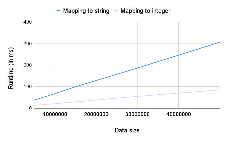
Both Query1 and Query2 give the same result, but Query2 is faster.
Prefer process operators over non-process equivalents
Sometimes process operators and non-process operators can be used to compute the same result. However, process operators are usually orders of magnitude faster.
Non-process operators | Process operators |
|---|---|
Choosing shorter expressions
Many conditional operators can be replaced with the CASE WHEN operator to achieve the same result. However, the specific operators have a reduced syntax that can help you make your PQL queries clean and understandable.
As a rule of thumb, you should always prefer shorter queries over longer ones, as this likely translates to better performance.
The GREATEST and LEAST operators offer a more concise syntax compared to CASE WHEN. In addition, they are a lot more intuitive if you have to compare more than two columns.
Example:
Query1 | GREATEST ( "Table1"."Column1" , "Table1"."Column2" ) |
|---|---|
Query2 | CASE WHEN "Table1"."Column1" >= "Table1"."Column2" THEN "Table1"."Column1" ELSE "Table1"."Column2" END |
With just two columns, Query2 is already twice as long as Query1. Adding more columns will increase the difference in length exponentially.
The COALESCE operator might be a good and more intuitive alternative to CASE WHEN statements for its reduced syntax.
Example:
Query1 | COALESCE ( "Table1"."Column1" , "Table1"."Column2" , 0 ) |
|---|---|
Query2 | CASE WHEN "Table1"."Column1" IS NOT NULL THEN "Table1"."Column1" WHEN "Table1"."Column2" IS NOT NULL THEN "Table1"."Column2" ELSE 0 END |
With only two columns, Query2 is more than twice as long as Query1.
Prefer PU-filter over CASE WHEN
When writing a PU function with a CASE WHEN as the input column where the ELSE section of the CASE WHEN returns a NULL, you can improve the performance by using the filter argument of a PU function instead.
The version with a filter argument is more performant, because it does not require creating a column for the CASE WHEN - requiring less memory and resulting in a faster execution.
Example:
Query1 | PU_SUM ( "Table1" , CASE WHEN "Table2"."Column1" IN ('a', 'b', 'c') THEN "Table2"."Column2" ELSE NULL END ) |
|---|---|
Query2 | PU_SUM ( "Table1" , "Table2"."Column2", "Table2"."Column1" IN ('a', 'b', 'c') ) |
Summary
Prefer | over |
|---|---|
COUNT | COUNT ( DISTINCT ) |
AVG | MEDIAN |
COUNT | SUM |
PU_COUNT | PU_COUNT_DISTINCT |
PU_AVG | PU_MEDIAN |
PU_COUNT | PU_SUM |
REMAP_VALUES | CASE WHEN |
= | LIKE |
IN | IN_LIKE |
mapping to integer | mapping to string |
process operators | non-process operators |
GREATEST / LEAST | CASE WHEN |
COALESCE | CASE WHEN |
PU-filter | CASE WHEN |
Being aware of expensive operations
Some complex PQL operators perform heavy computations and may require excessive CPU time. Being aware of such operators can help you distinguish the queries where a long runtime is unavoidable from the ones where investigating the query performance and optimizing it could be useful.
The following operators are generally considered expensive:
Note: If the execution time of some of the stated operators exceeds 10 minutes, the execution stops and an error is reported.
Key takeaways
These practices can enhance the performance of your dashboards and Apps:
Avoid overloading analyses sheets and views.
Use PU-functions to aggregate data into smaller tables.
Apply aggregations and FILTER_TO_NULL as "late" as possible.
Use less expensive standard aggregations.
Prefer less expensive operations.
Additional resources
For more details and examples you can refer to the Performance Optimization in PQL academy course.
For more information about the individual PQL operators you can refer to the PQL documentation.