LINK_PATH
Description
Warning
To use this feature, Object Link needs to be configured with Object Link in the data model.
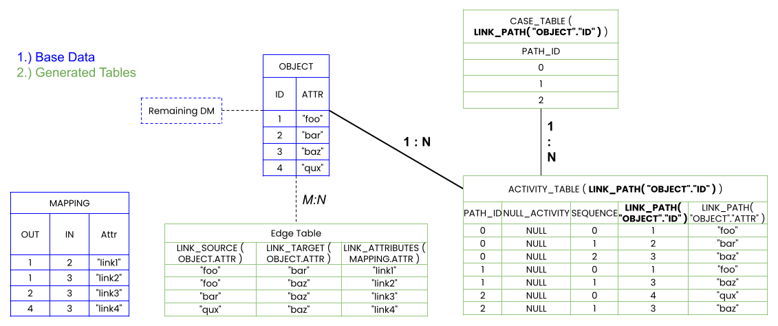
The LINK_PATH operator creates an internal activity and case table to represent individual paths calculated by traversing the Object Link graph. The resulting activity table is joined towards the input table and to the internal case table in a N:1 fashion. Additional tables containing link attributes are generated and can be accessed via the LINK_PATH_SOURCE/TARGET operators. An example of the created tables and how they are joined is shown below:
Warning
In some settings, this operator may require excessive CPU time. If the execution time exceeds 10 minutes, the execution is stopped and an error is reported.
The output of LINK_PATH is a column containing all objects of all calculated paths, where each row's data corresponds to the value of the object in the input column. If only individual objects are of interest and a complete path is not required, use LINK_SOURCE/LINK_TARGET instead. As the generated tables are joined to the input table, all objects, as specified in the Object Link mapping table, must reside within this one table in order to avoid join cycles in the data model. The underlying activity table generated by LINK_PATH is implicitly sorted by the SEQUENCE column within individual paths, indicated by the PATH_ID column.
Syntax
LINK_PATH ( input_table.column [, direction ] [, CONSTRAINED BY ( [ START ( start_objects_expression ) ] [, END ( end_objects_expression ) ] [, LENGTH ( comparison ) ] [, ALL ( all_objects_expression ) ] [, WITH/WITHOUT CYCLES] ) ] )
LINK_PATHacquires object attributes from the specifiedinput_table.column. Therefore, all objects, as they are specified in the Object Link mapping table, must be contained in this table. Entries of the input object table that are not mentioned in the mapping table are not legitimate objects for the Object Link graph and are ignored.directionspecifies the traversal direction. Valid values for the parameter areFORWARDS(default) andBACKWARDS.The graph traversal can further be
CONSTRAINED BY:start_objects_expressionis a condition to specify the start objects of the graph traversal.end_objects_expressionis a condition to specify the end objects of the graph traversal.comparisonis one of= X(equal),!= X(not equal),<> X(not equal),< X(less than),<= X(less than or equal),> X(greater than) or>= X(greater than or equal), whereXis a positive integer. This can be used to specify the desired path lengths (as measured by the number of objects). Another option isBETWEEN X AND Y, which means that the path lengths must be betweenXandY(inclusive).XandYmust both be positive integers andXmust be smaller than or equal toY.all_objects_expressionis a condition to specify which objects of the graph may be traversed.WITH CYCLESenables the traversal of cycles andWITHOUT CYCLESdisables the traversal of cycles. The default isWITHOUT CYCLES.
NULL handling
Object Link mapping table entries with NULL values in the IN or OUT column will register the object specified in the none-NULL entry. However, no link will be added to the Object Link graph.
NULL values in the
input_table.columnare retained in the output.
Scenario
The Object Link graph traversed by LINK_PATH can be arbitrarily complex and large. Formally, the graph is a directed multigraph, meaning that each link has a source and target object as well as an identity which allows multiple unique links between the same source and target pair. We refer to a group of links that share the same source and target objects as a multi-link. Additionally, the graph may contain cycles and self-loops. Objects therefore can appear multiple times within a path.
Warning
A multi-link may not consist out of more than 65'535 individual links. In the visualized graph below, one multi-link, from 'Egg' to 'Hard boiled eggs', exists with a quantity of 2.

Object Link graphs typically have objects that do not have INCOMING or OUTGOING links, these are called implicit START or END objects respectively and can also be found via the LINK_OBJECTS operator. In the illustration above, implicit START objects are indicated with an incoming link without a source and END objects are marked with a thick border.
This Object Link graph has the implicit start objects 'Olive oil', 'Flour' and 'Vegetables' and implicit end objects 'Veggie pasta', 'Chicken pasta' and 'Hard boiled eggs'. Note that 'Chicken' and 'Egg' are not implicit start objects as they each have an incoming link. These respective links form a cycle between those objects, however, a cycle can also be on one object itself, e.g. kneading object 'Dough' will again result in 'Dough'. This example graph also contains a multi-link for boiling eggs as we use different durations during the process.
Constraints
Parameters within the the CONSTRAINED BY clause are called constraints and control the traversal performed by LINK_PATH. They are intended to limit the result of the operator by specifying the critical areas within the graph. Also see the chapter about "Why does LINK_PATH hit the table row limit?". Each constraint may only appear once but can otherwise be freely combined with each other.
Unconstrained
A LINK_PATH call that does not specify any constraints is called unconstrained and has the following default behavior:
STARTconstraint: Use implicitSTARTobjects of the Object Link graph.ENDconstraint: Use implicitENDobjects of the Object Link graph.LENGTHconstraint: Use defaultLENGTHlimit of 10. A warning will be emitted if longer paths exist.ALLconstraint: AllowALLobjects to be traversed.CYCLESconstraint: Enable/Disable cycles to be traversed.
[1] The | ||||||||||||||||||||||||||||||||||||||||||||||||||||||||||||||||||||||||||||||||||||||||||||||||||||||||||||||||||||||||||||||||||||||||||||||||||||||||||||||||||||||||||||||||||||||
| ||||||||||||||||||||||||||||||||||||||||||||||||||||||||||||||||||||||||||||||||||||||||||||||||||||||||||||||||||||||||||||||||||||||||||||||||||||||||||||||||||||||||||||||||||||||
|
[2] Besides the activity table, | |||||||||||||||||||||||||||||||||||||||||||||||||||||||||||||||||||||||||||||||||||||||||||||||||||||||||||||||||||||||||||||||||||||||||||||||
| |||||||||||||||||||||||||||||||||||||||||||||||||||||||||||||||||||||||||||||||||||||||||||||||||||||||||||||||||||||||||||||||||||||||||||||||
|
[3] The resulting | |||||||||||||||||||||||||||||||||||||||||||||||||||||||||||||||||||||||||||||||||||||||||||||||||||||||||||||||||||||||||||||||||||||||||||||
| |||||||||||||||||||||||||||||||||||||||||||||||||||||||||||||||||||||||||||||||||||||||||||||||||||||||||||||||||||||||||||||||||||||||||||||
|
Direction
Traversal in LINK_PATH can be either FORWARDS (default) OR BACKWARDS.
[4] So far we've only seen the default | |||||||||||||||||||||||||||||||||||||||||||||||||||||||||||||||||||||||||||||||||||||||||||||||||||||||||||||||||||||||||||||||||||
| |||||||||||||||||||||||||||||||||||||||||||||||||||||||||||||||||||||||||||||||||||||||||||||||||||||||||||||||||||||||||||||||||||
|
START and END
Traversal of the Object Link graph can be defined by specifying conditions on the input_table. Conditions in the START constraint specify where the traversal begins and the END constraint indicates where a path is finished. Note while specifying these constraints that the conditions are not automatically combined with the implicit START or END objects. If the implicit objects without INCOMING or OUTGOING links shall be used with additional conditions, we can utilize the LINK_OBJECTS operator to explicitily formulate the implicit objects.
[5] By specifying only 'Egg' as a | ||||||||||||||||||||||||||||||||||||||||||||||||||||||||||||||||||||||||||||||||||||||||||||||||||||||||||||||||||||||||||||||||||||
| ||||||||||||||||||||||||||||||||||||||||||||||||||||||||||||||||||||||||||||||||||||||||||||||||||||||||||||||||||||||||||||||||||||
|
[6] In the following example, we specify implicit | |||||||||||||||||||||||||||||||||||||||||||||||||||||||||||||||||||||||||||||||||||||||||||||||||||||||||||||||||||||||||||||||||||
| |||||||||||||||||||||||||||||||||||||||||||||||||||||||||||||||||||||||||||||||||||||||||||||||||||||||||||||||||||||||||||||||||||
|
LENGTH
Arbitrarily long paths could result from traversal on an Object Link graph. To allow and disallow paths of certain lengths we can make use of the LENGTH constraint.
[7] In this example, we only want paths whose length (as measured by the number of involved objects) is equal to 2. | |||||||||||||||||||||||||||||||||||||||||||||||||||||||||||||||||||||||||||||||||||||||||||||||||||||||||||||||||||||||||||||||
| |||||||||||||||||||||||||||||||||||||||||||||||||||||||||||||||||||||||||||||||||||||||||||||||||||||||||||||||||||||||||||||||
|
ALL
Thanks to the ALL constraint, we can guarantee that all objects in the resulting paths fulfill a certain condition.
[8] If we want every path that does not involve traversing certain objects, we can avoid them via the | |||||||||||||||||||||||||||||||||||||||||||||||||||||||||||||||||||||||||||||||||||||||||||||||||||||||||||||||||||||||||||||||
| |||||||||||||||||||||||||||||||||||||||||||||||||||||||||||||||||||||||||||||||||||||||||||||||||||||||||||||||||||||||||||||||
|
CYCLES
With the cycles constraint we can enable or disable the traversal of cycles in the created graph. A cycle is detected when any object would occur twice within one traversed path. WITHOUT CYCLES is set by default, so that no cycles are traversed.
[9] With cycles enabled, we get additional paths that contain the self-link on 'Dough'. | |||||||||||||||||||||||||||||||||||||||||||||||||||||||||||||||||||||||||||||||||||||||||||||||||||||||||||||||||||||||||||||||||||||||
| |||||||||||||||||||||||||||||||||||||||||||||||||||||||||||||||||||||||||||||||||||||||||||||||||||||||||||||||||||||||||||||||||||||||
|
Why does LINK_PATH hit the table row limit?
When the LINK_PATH operator traverses a large Object Link graph, it stores the paths it finds as rows in a table. If this table becomes too large, an error is returned indicating that the table row limit has been reached. To demonstrate how quickly the number of paths can grow, let's look at a simple example production process for making chocolate strawberry cake, as shown in the following figure.
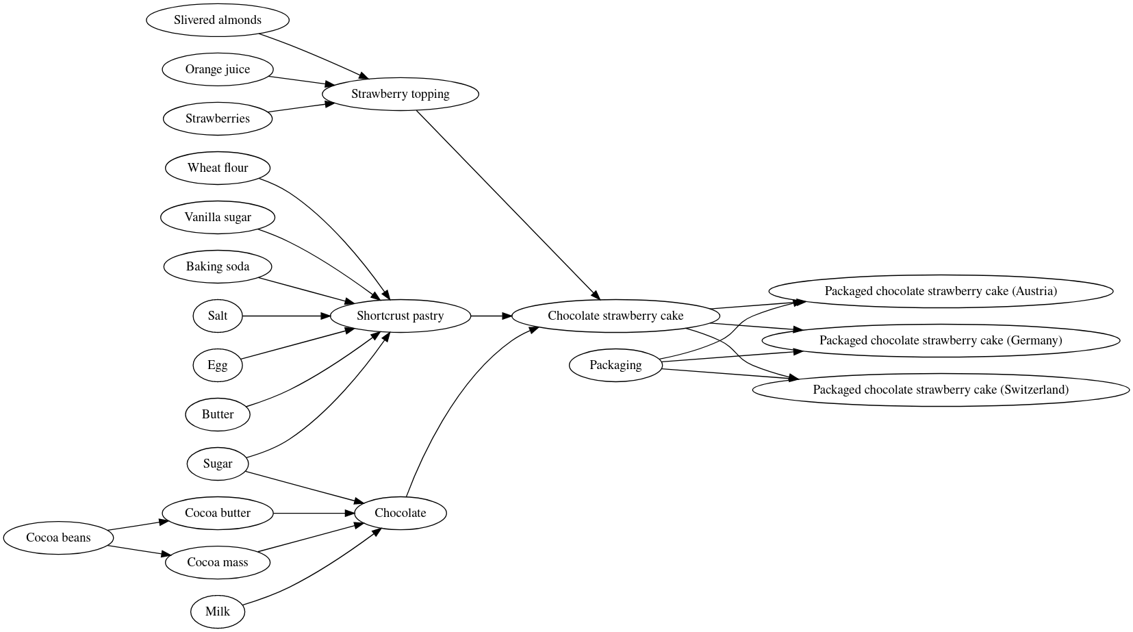
When this Object Link graph is traversed without constraints using the query below, the result consists of 45 paths and 180 rows, which is quite a lot for such a small graph.
LINK_PATH ( "Materials"."Description" )
However, if our use case does not require packaged cakes, we can add a constraint to stop traversing the graph when we reach the unpackaged chocolate strawberry cake as shown in the following query. This drastically reduces the size of the result, which is now only 14 paths and 44 rows. That's three times fewer paths and four times fewer rows just by omitting three packaged cakes. In real processes with thousands of objects and links, the number of paths will grow even faster. Therefore, it is critical to limit the traversal of the Object Link graph to only those objects that are essential to a use case.
LINK_PATH ( "Materials"."Description" , CONSTRAINED BY ( END ( "Materials"."Description" = 'Chocolate strawberry cake' ) ) )
The following figure gives a rough indication of when the table row limit might be reached for Object Link graphs of different sizes if no constraints are used. For example, for an Object Link graph with 10,000 objects, the table row limit is likely to be reached when the number of links exceeds 26,000. In general, we strongly recommend the use of constraints once the ratio of links to objects is greater than 2.
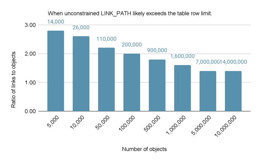
Use the following queries to calculate the number of links, the number of objects, and the ratio of links to objects for your Object Link graph.
COUNT ( LINK_SOURCE ( table.column ) )
COUNT_TABLE ( LINK_OBJECTS ( table.column ) )
COUNT ( LINK_SOURCE ( table.column ) ) / GLOBAL ( COUNT_TABLE ( LINK_OBJECTS ( table.column ) ) )
Advanced Examples
[10]
This example further illustrates how including cyclic paths easily blows up the result even though only a few objects are involved. | ||||||||||||||||||||||||||||||||||||||||||||||||||||||||||||||||||||||||||||||||||||||||||||||||||||||||||||||||||||||||||||||||||||||||||||||||
| ||||||||||||||||||||||||||||||||||||||||||||||||||||||||||||||||||||||||||||||||||||||||||||||||||||||||||||||||||||||||||||||||||||||||||||||||
|
[11] The result of | |||||||||||||||||||||||||||||||||||||||||||||||||||||||||||||||||||||||||||||||||||||||||||||||||||||||||||||||||||||||||||||||||||||
| |||||||||||||||||||||||||||||||||||||||||||||||||||||||||||||||||||||||||||||||||||||||||||||||||||||||||||||||||||||||||||||||||||||
|