Join functionality
Description
Celonis performs implicit joins when a query accesses several tables. This means that the user does not have to define the join as part of a query, but the tables are joined as defined in the Data Model Editor.
Implicit joins
[1] Here ActivityTable and CaseTable are queried. The customer information of the CaseTable is implicitly joined to the activities of the ActivityTable: 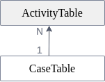 Joins are always executed as left outer equi joins. In this example the ActivityTable is on the left side of the join. Therefore the activity D, which doesn't have a join partner in the case table, is part of the result, while Case ID 4 is not. Also it is noteworthy that NULL values are never joined, as it is the case for activity E. It depends on the join cardinality which table is on the left side of the join. Celonis supports 1:N relationships. 1:N relationships means that if for example Table A and B are joined together, every row in B can have zero or one join partner in table A, but not more. There is no limitation in the other direction. Every row in A can have an arbitrary number of join partners. In N:1 relationships, Celonis automatically detects the table on the N-side based on the loaded data. 1:1 relationships are not natively supported, but are treated as a special case of a 1:N relationship. N:M joins are not supported because they are rare, because they can be transformed into simpler relationships by adding a mapping table in between the two tables, and because they would make it much harder to understand the result. The N-side is always put on the left side of the join. In this example, it is easy to see that case 1 and case 2 have two join partners in the activity table, while every activity relates to exactly one case. Therefore the ActivityTable is on the left side of the join. In other words, ActivityTable is the fact table, and CaseTable is the dimension table in that join. These terms are explained in more detail below. | ||||||||||||||||||||||||||||||||||||||||||||
| ||||||||||||||||||||||||||||||||||||||||||||
|
Join relationships
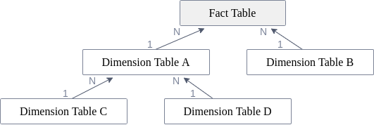
It is not possible to join every table to any other table within a data model. Celonis supports an extended snowflake schema for a data model. A snowflake schema consists of one fact table which can have multiple N:1 relationships to dimension tables. These dimension tables can themselves have N:1 relationships to other tables. Celonis extends the classic snowflake schema by supporting multiple fact tables, but no cyclic join graphs. To resolve a cyclic join graph you may have to add a table several times to the data model.
The following join graph shows an example of a snowflake schema:
This Wikipedia article provides more information on the snowflake schema.
The common table
To process a join, we first identify the common table. In general, the common table of two tables A and B is the table on the N-side among all tables in between A and B, including A and B themselves.
In the above example schema, for Dimension Table C and Dimension Table D, the Dimension Table A is identified as the common table, because it is the table on the N-side between the two tables. This means that if a column from Dimension Table C should be joined with a column from Dimension Table D, Celonis identifies the Dimension Table A as the common table. It then joins the needed columns from Dimension Table C and Dimension Table D to the Dimension Table A. We call this step pulling up the data.
The common table of two tables does not need to be a third table in between, but can also be one of those two tables. In the above example schema, for Dimension Table C and the Fact Table, the Fact Table is identified as the common table because it is the table on the N-side of the join graph between the involved tables.
This works perfectly as long as you have only one possible table on the N-side of the join graph. If you have multiple tables on the N-side, it is not possible to identify a single common table for your join.
The following example schema shows this situation:
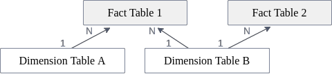
In this example, there is no common table for Fact Table 1 and Fact Table 2, because both tables are on the N-side of the join graph. The same holds for Dimension Table A and Fact Table 2. Please note that all other table combinations do have a common table, i.e.
Dimension Table AandDimension Table B(common table:Fact Table 1),Dimension Table AandFact Table 1(common table:Fact Table 1),Dimension Table BandFact Table 1(common table:Fact Table 1),Dimension Table BandFact Table 2(common table:Fact Table 2).
Understanding the "No common table" error message
In Celonis, two tables can only be joined when they have a common table. So if all tables which are used inside a query do not have a common table, they cannot be joined together, and the following error is returned:
Warning
No common table could be found. The tables ["Fact Table 1"] and ["Fact Table 2"] are connected, but have no common table. This means that they do not have a direct (or indirect) 1:N or N:1 relationship. Join path: [Fact Table 1]N <-- 1![Dimension Table B]!1 --> N[Fact Table 2]. For more information on the join path, search for "Join functionality" in PQL documentation.
As mentioned, the join graph is acyclic, which means there is exactly one join path between any two connected tables. In cases where no common table can be determined between two connected tables, the join path is also shown in the error message (see above). The join path contains the following information:
Table name:
[Fact Table 1]A table surrounded by exclamation marks breaks the possibility of a common table:
![Dimension Table B]!Join direction:
-->or<--Join cardinalities:
1 --> NorN <-- 1
Understanding the warning "The aggregation function [...] is applied on a column from table [...] which has a 1:N relationship to the common table [...]"
Executing the join, i.e. pulling up all data to the common table, is done before executing the standard aggregations. Consequently, aggregation inputs also contribute to the common table. Executing the join before the aggregations means that an aggregation can be executed on a column that has been pulled up, potentially taking the same origin value into account multiple times.
The following example schema showcases this situation:
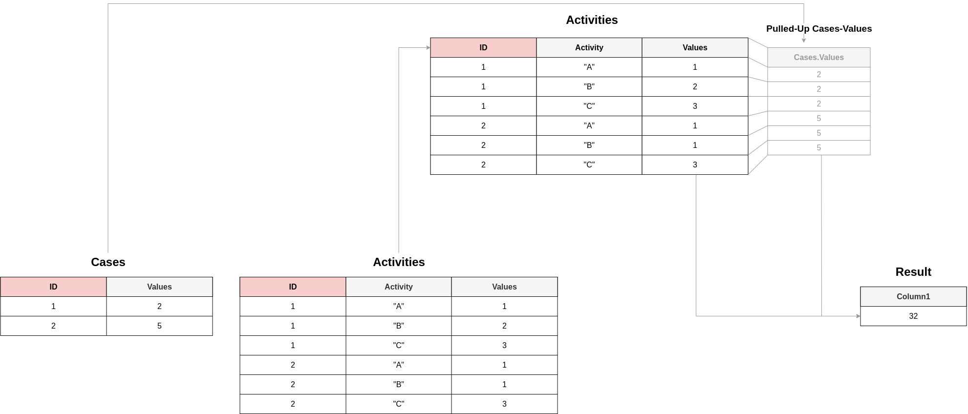
In this scenario SUM(Cases.Values) would result in a table containing the value 7 and SUM(Acitivities.Values) would result in a table containing the value 11. So it might be assumable that SUM(Cases.Values)+SUM(Acitivities.Values) could (falsely) lead to a table containing the value 18, but - as before mentioned - the values of Cases.Values get pulled up (visualiuzed in grey) to their common table (i.e., the "Activities"-table) and lead to the actual result of 32. In that case, the following warning is emitted to make the user aware of the implicit join in those cases:
Warning
The aggregation function AGG is applied on a column from table "DimensionTable" which has a 1:N relationship to the common table "FactTable". This means that one input value can contribute to the aggregation result multiple times. For more information search for "Join functionality" in PQL documentation.
While the query can still be valid and calculate the correct results even if the warning is displayed, in most cases it is a hint that the query does not calculate what the user intended. There are multiple ways to fix the query and get rid of the warning accordingly. The following subsections show examples of the most frequent pitfalls and possible solutions.
Multiple KPI calculations per Query
When introducing the join to another table inside one KPI, this join affects all other dimensions and KPIs of that particular query. Take a look at the following three-part example:
[2] This query calculates the average throughput time using the CALC_THROUGHPUT function. Since case 1 has a throughput time of 8 days, and case 2 has a throughput time of 2 days, we get the expected result of 5 days: | ||||||||||||||||||||||||||||||||
| ||||||||||||||||||||||||||||||||
|
[3] Now we add another KPI to our query. It should count the overall number of D-activities. As you can see, the result of the throughput time calculation is now 6 days, although the formula for this KPI and the input data did not change. The result of CALC_THROUGHPUT is on case level (i.e. the throughput time is calculated per case). This means that when we only use However, when adding the KPI counting the D-activities, the join to the Activity table is introduced, which means that all columns of the Case table (including the | ||||||||||||||||||||||||||||||||||
| ||||||||||||||||||||||||||||||||||
|
[4] To get the expected values for both KPIs while having them inside the same query, we could get rid of the join with the Activity table again by calculating the number of D-activities for each case first in a PU_COUNT. As we specify the Case table as the target table of the PU function, the result of the PU function belongs to the Case table rather than the Activity table: | ||||||||||||||||||||||||||||||||||
| ||||||||||||||||||||||||||||||||||
|
Single KPI consisting of multiple aggregations
Imagine you have two single KPIs (i.e. two aggregations without groupers) in different components, and you would like to combine them into one KPI (e.g. adding or dividing them). If they are based on different tables, you might not get the same result as if you would combine their results from executing inside the same component. Take a look at the following example:
[5] In this example, we simply count the total number of Activities. As expected, we get 6 as a result: | ||||||||||||||||||||||||||||||||
| ||||||||||||||||||||||||||||||||
|
[6] Similar to the first query, we also calculate the total number of Cases in a separate query. We get 2, which is the result that we expect: | ||||||||||||||||||||||||||||||||
| ||||||||||||||||||||||||||||||||
|
[7] Now let's assume we want to calculate the average number of Activities per Case. One way of calculating this would be to take the total number of Activities and divide it by the total number of Cases. As calculated before, the total number of Activities is 6, and the number of Cases is 2, therefore we expect an average of 3 Activities per Case. But here we have to be careful: We cannot simply take the PQL formulas from before which calculate both counts and divide them as shown in this example. Since both single KPIs are based on different tables, the inputs are first brought to the common table before evaluating the aggregations. The consequence is that the count of the cases does not return 2 anymore in this context, but 6, because the CASE_ID column of the Case table has 6 rows after pulling it up to the Activity table (which is the common table). In the end, we essentially calculate 6/6, which is 1. The warning that this query might not calculate the intended value is also shown: | ||||||||||||||||||||||||||||||||
| ||||||||||||||||||||||||||||||||
|
[8] For aggregations without grouping, the desired behavior can usually be achieved by using the GLOBAL function. GLOBAL gives the possibility to execute the provided aggregation in an "isolated" manner from the rest of the query - the aggregation does not influence the common table and no pull-ups happen. The result of GLOBAL behaves like a constant. It would be enough to only wrap the aggregations on the tables which are not the common table into a GLOBAL function, but it is easiest to simply always apply it. Due to the GLOBAL, both counts are evaluated separately, and then the resulting constants (6 activities and 2 cases) are divided. There is no warning message shown anymore, and the expected result (3) is returned: | ||||||||||||||||||||||||||||||||
| ||||||||||||||||||||||||||||||||
|