Vertica SQL performance optimization guide
When looking to optimize your Vertica SQL performance, we recommend the following:
When creating transformation queries, every choice has an impact on performance. Understanding the impact gives us the possibility to apply the best practices, avoid anti-patterns and improve overall query performance.
Every transformation (data preparation and cleaning) in the Celonis Event collection module is executed in a Vertica database. For each query submitted to Vertica, the query optimizer assembles a Query Execution Plan. A Query Execution Plan is a set of required operations for executing a given query. This plan can be accessed and analyzed by adding the EXPLAIN command to the beginning of any query statement, as seen in the following example:
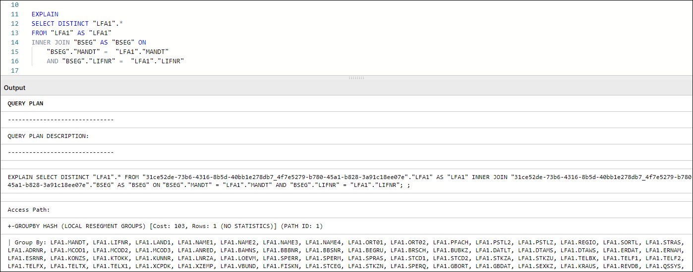
Figure 1: Query Plan Example in Vertica
The complexity of the query will determine the variety of information contained in the Query Plan. In most cases, our checks on query performance focus on specific areas as expanded in the following sections of the guide.
For use with tables containing 10,000 or more records
You should only create statistics for tables that have 10,000 records or more. The effort required to create statistics for tables with fewer than 10,000 is greater than the time saved by using them.
Table Statistics are analytical summaries of tables that assist the query optimizer in making better decisions on how to execute the tasks involved with the query. They provide information about the number of rows and column cardinality in the table.
In tasks such as SELECT, JOIN, GROUP BY, the plan will indicate whether a table has statistics available or not for the execution of query tasks.
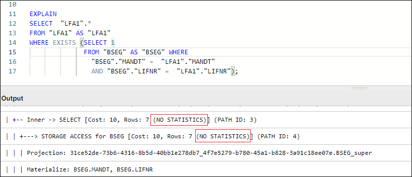
Figure 2: Example Query Plan showing NO STATISTICS for BSEG table
By default, Table Statistics are automatically updated for all raw tables extracted from the source system via Celonis Extractor (e.g. VBAK, EKKO, LIPS).
However, any temporary or other tables created and used in Transformations will not have table statistics refreshed by default. Missing Table Statistics will impact all downstream transformations that use the tables, as well as Data Model loading times in some cases. To ensure optimal performance, an ANALYZE_STATISTICS command should be executed when creating any table via Transformations.
Users can check which tables in their schema do not have Statistics refreshed by running the following query:
SELECT anchor_table_name AS TableName

FROM projections

WHERE has_statistics =FALSE ;
If this query returns any result, a SELECT ANALYZE_STATISTICS ('TABLE_NAME'); should be added in the transformation script that creates the respective table and database will gather table statistics when the query/transformation is executed.
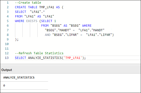
Figure 3: Example Table Creation & Table Statistics Refresh, with typical SQL Workbench output
In SQL, DISTINCT is a very useful command when needing to check or count distinct values in a field, or deduplicate records in smaller tables. While the use of DISTINCT in such cases is necessary, many users resort to DISTINCT (eg SELECT DISTINCT *) often times as a quick fix to remove duplicate records that result from the following scenarios:
Bad Data Quality: The extraction of the source table has quality issues that show up as duplicate records. These issues, if they exist, should be addressed at a source system/extraction level.
Use of DISTINCT to limit table population: A join is performed between two or more tables to limit the scope of the table content to only entries relating to records that exist in another table (e.g. AP_LFA1 Data model table is table LFA1 limited to Vendors who appear in AP Invoice Items).
In Vertica specifically, DISTINCT works as an implied GROUP BY, as can be seen in Figure 1. In that example, the GROUPBY HASH task has a significant cost proportionally to the total cost and is used to limit the LFA1 table population. In such cases, we suggest avoiding the use of DISTINCT and finding alternative ways to avoid the duplication caused by using JOIN to limit LFA1, and using WHERE EXISTS instead.
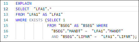
Figure 4: Example using WHERE EXISTS instead of JOIN + SELECT DISTINCT
How do temporary join tables affect Transformation performance?
When creating temporary join tables, users should think about the purpose of the table and its relations with other tables (joins). In that respect, a well-designed temporary table:
Has a clear purpose, for example, to pre-process or join data, filter out irrelevant records, calculate certain columns that will be used later in transformations, etc. The sense of purpose should be validated, so as to confirm that the creation of temporary tables has a positive impact on overall performance.
Contains only necessary data (e.g. only really required columns and records).
Is sorted by the columns most often used for joins with other tables (e.g., MANDT, VBELN, POSNR). To ensure the proper sorting of the table, put those columns at the beginning of the create table statement or add an explicit ORDER BY clause at the end of the statement.
Doesn’t contain custom/calculated fields in the first column(s). As shown in the example below, the first columns should be the ones that are used for joins (key columns). If this is not the case, Vertica will have to perform additional operations (e.g. creating hash tables) while running the queries, which will extend the execution time.
In the example below, auxiliary table O2C_VBAK_VBAP is being defined with an improper column order. This in turn will cause the table to be sorted by the fields in the order they appear in the SELECT statement. The expected use case of this table involves joins on VBAK key fields (MANDT, VBELN, POSNR) which are not the fields that are part of the table sorting. In such a use case and with the definition of the table as seen on the left side, the joins to this table will not be performed optimally.
The correct definition for the table should have the table fields ordered initially with the table keys, then any other custom keys that may be used in joins, followed by calculated and other fields, as see on the script example on the right. This will ensure that the table is sorted by the fields that are used as condition joins and will result in a more efficient execution plan when joining to this table. In most cases, that would be a MERGE JOIN.
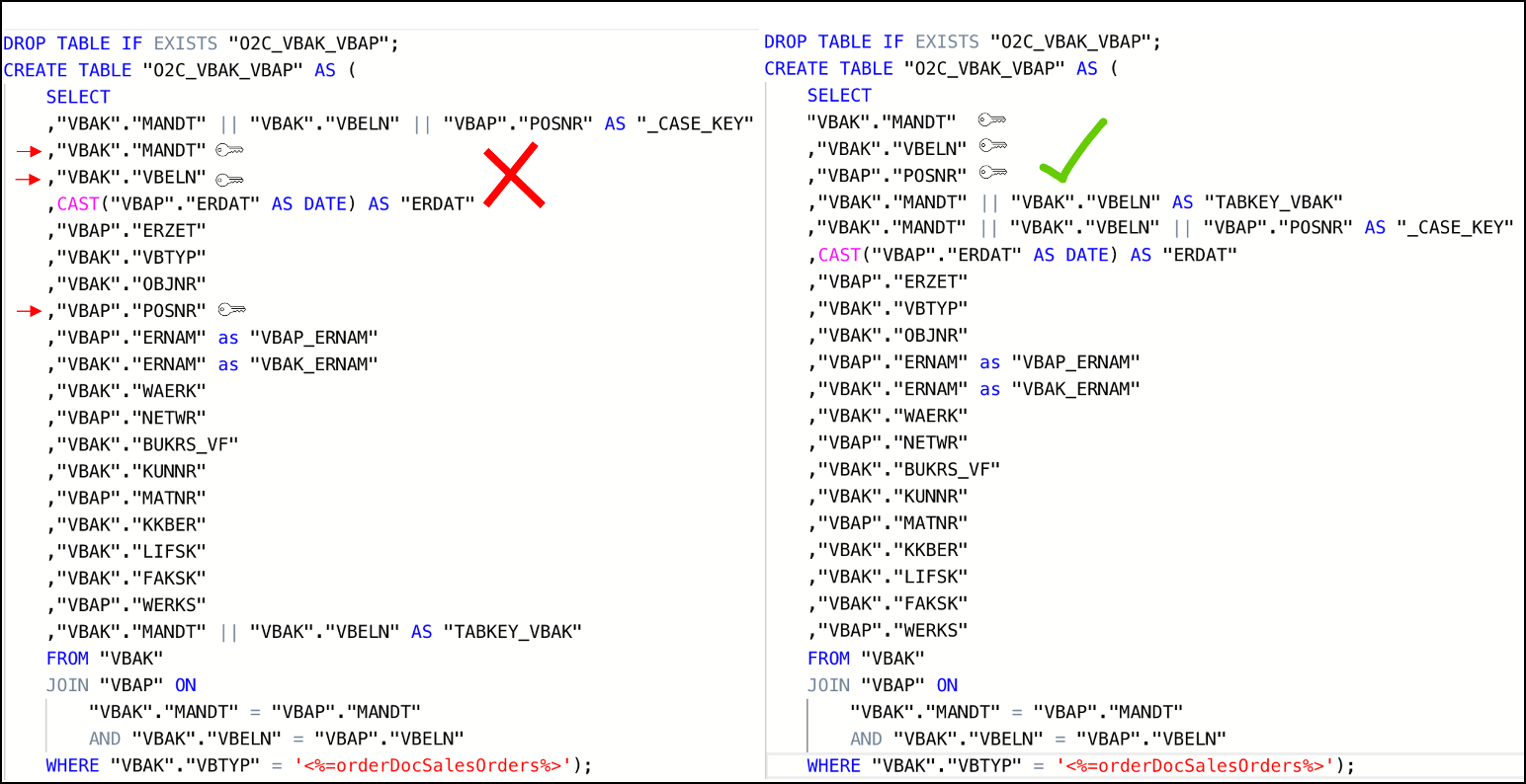
Figure 5: Example Scripts of poorly designed temporary table (left) vs well-designed temporary table (right)
Alternatively, an explicit ORDER BY can be used when creating a table in order to force a specific ordering of the new temporary join table.
Note
MERGE and HASH Joins
Vertica uses one of two algorithms when joining two tables:
Hash Join - If tables are not sorted on the join column(s), the optimizer chooses a hash join, which consumes more memory because Vertica has to build a sorted hash table in memory before the join. Using the hash join algorithm, Vertica picks one table (i.e. inner table) to build an in-memory hash table on the join column(s). If the table statistics are up to date, the smaller table will be picked as the inner table. In case statistics are not up to date or both tables are so large that neither fits into memory, the query might fail with the “Inner join does not fit in memory” message.
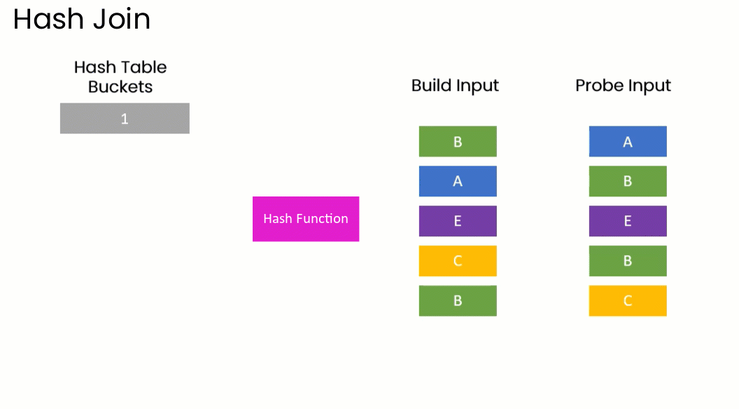
Merge Join - If both tables are pre-sorted on the join column(s), the optimizer chooses a merge join, which is faster and uses considerably fewer resources.

So which join type is appropriate?
In general, aim for a merge join whenever possible, especially when joining very large tables.
In reality, transformation queries often contain multiple table joins. So, it's rarely feasible to ensure that all tables are joined as a merge type because it requires tables to be presorted on join columns.
A merge join will always be more efficient and use considerably less memory than a hash join. But it's not necessarily faster. If the data set is very small, a hash join may process faster but this is very rare.
Alongside the creation of a well-designed temporary table, it is also essential to make sure that two tables are adequately joined by the entire join predicates (keys). For example, the MANDT (Client) column is often unduly excluded from join predicates which can have a very negative impact on query performance, ignoring potential MERGE JOIN even when both data sets are properly sorted, as seen in the following example:
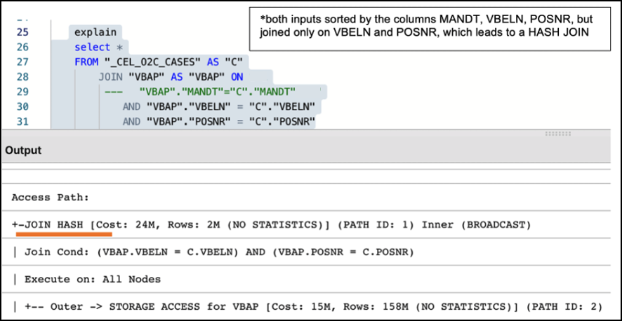
Figure 6: Example of Performance Impact between using partial and entire keys when joining tables
Note
What are Projections?
Unlike traditional databases that store data in tables, Vertica physically stores table data in projections. For every table, Vertica creates one or more physical projections. This is where the data is stored on disk, in a format optimized for query execution.
The projection created needs to be sorted by the columns most frequently used in subsequent joins (usually table keys), because the projection sorting acts like indexes do in Oracle SQL or SQL Server. The sorting of the underlying table projection is why users are encouraged to properly structure and sort their tables, as described in the section above.
Currently, two projections are used in Celonis Vertica Databases for extracted tables:
Auto-projection (super projection) created immediately on table creation. It includes all table columns and is sorted by the first 8 fields, at the order they are exported.
If the primary key is known (set up in the table extraction setting), Vertica creates additional projections sorted by and containing only the primary key fields. Such projections may be used by Vertica for JOIN or EXIST operations.
The performance of all queries that use temporary/auxiliary tables (i.e. all tables created during transformation) will heavily depend on the super-projection that is created by Vertica at the time of the table’s creation. By default, Vertica sorts the default super-projection by the first 8 columns as defined in the table definition script.
Additional read:
Using views instead of tables might negatively impact transformations and data model load performance. While a temporary table stores the result of the executed query, a view is a stored query statement that has to be executed every time it is invoked.
Aspect | View | Table |
|---|---|---|
When it is executed | During data model loads. | During transformations. |
Persistence | Is saved in memory. | Is persisted to storage. |
Life cycle | Resulting dataset is dropped after the query which called it no longer needs it. | Is dropped when a DROP TABLE statement is executed. |
When to use |
|
|
Common mistakes | Nested views – a query can call a view, which calls another view. This causes poor performance and a high risk of errors. | Poor design – the first columns of such tables should be primary/foreign keys in subsequent transformations (to promote merge joins over hash joins). |
Statistics | Views cannot have own statistics – query planner uses statistics of underlying tables. | Tables can (and should) have own statistics. |
Sorting | Do not have own sorting, uses sorting of underlying tables. | Can have own sorting – if sorted on columns used for joins, promotes more performant merge joins. |
All things considered, one should analyze the specific scenario, ideally, test both approaches and choose the one which is more performant in terms of total transformation and data model load time.
Implementing Staging Tables for Data Model
For every source table that is needed to be present in the Data Model (eg. VBAP), the standard approach is to define a table or view (e.g. O2C_VBAP), with all VBAP fields (VBAP raw data), as well as additional calculated/converted fields that will be needed for analyses (VBAP Transformed Data). In instances of large transactional tables such as VBAP, a user may face the following dilemma:
Define O2C_VBAP as a Table: The table will be loaded faster in the Data Model, but the Transformation defining it will be running longer than defining a view. APC consumption will also be increased, as all VBAP columns will need to be stored twice, once in the source table (VBAP) and another in the Data Model Table (O2C_VBAP).
Define O2C_VBAP as a View: The definition in the Transformation will only need seconds to run and there will not be an impact on APC. However, Data Model load runtimes will increase, as the view will need to be invoked and run and its resulting set will then need to be loaded in the Data Model.
While both scenarios above have their pros and cons, and some users may be satisfied with those based on their use case and data size, the most optimal way is to use both View and Table structures, to leverage the advantages of both, and balance savings in APC as well as reductions in overall runtime.
When defining the Staging Table, VBAP keys (MANDT, VBELN, POSNR) should be selected first. The statement should also include all the joins and functions required to define the Transformed Data fields (calculated fields). The users now have a table structure containing all additional fields for VBAP data model table, without having to store the rest of the original VBAP fields twice, which results in reduced APC consumption.
Subsequently, a data model view is created (e.g. O2C_VBAP), which joins the “raw data” table (i.e. VBAP) with the transformed data table (i.e. O2C_VBAP_STAGING). As the two tables (VBAP and Staging) are joined on keys and it is the only join taking place during the Data Model load, the materialization of the view is much more performant.
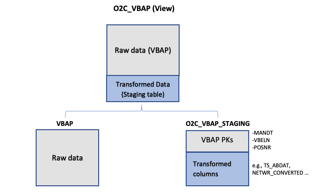 |
Figure 7: Leveraging Staging Tables in Data Model. In this example, View O2C_VBAP is based on a join between the existing source table (VBAP) and O2C_VBAP_STAGING table.
Important
A common problem with long running transformations and slow data model loads is due to missing statistics in Vertica. This issue can be resolved by adding the Vertica ANALYZE_STATISTICS statement directly in the SQL. For more information, refer to Vertica Transformations Optimization.
Example: Staging Table Definition (O2C_VBAP_STAGING):
CREATE TABLE "O2C_VBAP_STAGING" AS
(
        SELECT

        "VBAP"."MANDT", --key column
                "VBAP"."VBELN", --key column
                "VBAP"."POSNR", --key column
        CAST("VBAP"."ABDAT" AS DATE) AS "TS_ABDAT",
        IFNULL("MAKT"."MAKTX",'') AS "MATNR_TEXT",
        "VBAP_CURR_TMP"."NETWR_CONVERTED" AS "NETWR_CONVERTED",
        "TVRO"."TRAZTD"/240000 AS "ROUTE_IN_DAYS"
        FROM "VBAP" AS "VBAP"
        INNER JOIN "VBAK" ON
            "VBAK"."MANDT" = "VBAP"."MANDT"
                    AND "VBAK"."VBELN" = "VBAP"."VBELN"
                AND "VBAK"."VBTYP" = '<%=orderDocSalesOrders%>'
        LEFT JOIN "VBAP_CURR_TMP" AS "VBAP_CURR_TMP" ON
            "VBAP"."MANDT" = "VBAP_CURR_TMP"."MANDT"
                AND "VBAP"."VBELN" = "VBAP_CURR_TMP"."VBELN"
                AND "VBAP"."POSNR" = "VBAP_CURR_TMP"."POSNR"
                LEFT JOIN "MAKT" ON
                "VBAP"."MANDT" = "MAKT"."MANDT"
                        AND "VBAP"."MATNR" = "MAKT"."MATNR"
            AND "MAKT"."SPRAS" = '<%=primaryLanguageKey%>'
            LEFT JOIN "TVRO" AS "TVRO" ON
                        "VBAP"."MANDT" = "TVRO"."MANDT"
                        AND "VBAP"."ROUTE" = "TVRO"."ROUTE"
);
Example: Data Model View Definition (O2C_VBAP):
--In this view the only one join, between the raw table (VBAP) and the staging table (O2C_VBAP_STAGING) is performed. All other joins, required for calculation of the fields should be part of the STAGING_TABLE statement

CREATE VIEW "O2C_VBAP" AS (
        SELECT
        "VBAP".*,
                "VBAP_STAGING"."TS_ABDAT",
                "VBAP_STAGING"."MATNR_TEXT",
                "VBAP_STAGING"."TS_STDAT",
                "VBAP_STAGING"."NETWR_CONVERTED",
                "VBAP_STAGING"."ROUTE_IN_DAYS",
        FROM "VBAP" AS "VBAP"
        INNER JOIN "O2C_VBAP_STAGING" AS VBAP_STAGING ON
            "VBAP"."MANDT" = "VBAP_STAGING"."MANDT"
                    AND "VBAP"."VBELN" = "VBAP_STAGING"."VBELN"
                AND "VBAP"."POSNR" = "VBAP_STAGING"."POSNR"
);
Nested Views and Performance
In many cases, the use of nested views can affect performance, especially when used in Data Model views. While views are useful when wanting to run simple statements (such as SELECT) on a pre-defined result set, they should not be interchangeable with table structures in their usage. When dealing with transaction data (ie the larger data sets), we discourage users from performing transformation queries that join multiple views together, or using views in the definition of (Data Model or other) views, similar to the structure below:
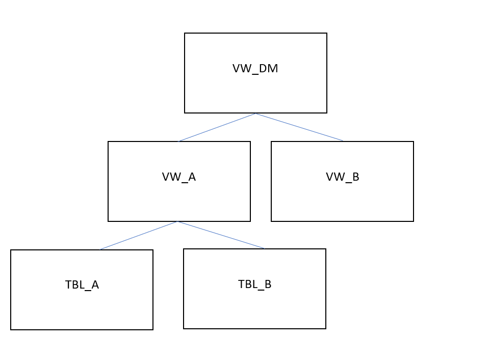 |
Figure 8: Example of Nested Views in a Data Model View Definition
In this example. View A is defined by a transformation that uses Tables A and B. View A is then joined to View B in the transformation that defines the Data Model View. When the Data Model View is invoked during the Data Model Load, VW_DM will have to be materialized at that stage, which includes running all the following tasks:
The transformation query that creates VW_A will be executed.
The transformation query that creates VW_B will be executed.
The transformation query that creates VW_DM will be executed.
The execution of all those steps/tasks together will greatly affect Data Model Load performance. In addition to that, any tasks that use views instead of tables, in our case the definition of VW_DM, will not be able to use projections, table sorting or table statistics, thus making the data model load execution even slower. This problem compounds as users add more view layers and more numbers of joins between views in order to reach their desired output.
In such cases, we strongly suggest the use of auxiliary/temporary tables in intermediary transformation steps, with their table statistics fully analyzed. Auxiliary tables can then be dropped as soon as they are no longer needed for further transformations. In our example above, Views VW_A and VW_B, as well as View VW_DM, should be created as tables instead, with VW_A and VW_B being dropped right after VW_DM is created.